Measuring Object Length (with a Reference Object)

It has been a long long time I've not update this blog due to my new notebook modem spoiled just after I bought it! The support staff came 3 times and now I am waiting for a replacement model...

Further more, life become more and more busy, and sometimes I really out of idea what to post here. :P

Until I receive some e-mail from some reader...

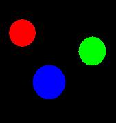
This is rather a simple example to measure a length of an object in an image. We could easily get the reading in pixels, and with a reference, we could just use a simple mathematic to compute the lenght in some standard unit.

Let's see this simple example:

1. Reading image and show the true color image.
clear all;clc;
I = imread('pic29.tif');
imshow (I);



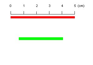
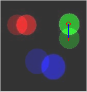
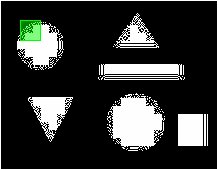
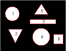
2. Assuming that we know the length of the red object (as reference) which is 5 cm, locate the red object with simple command and find the length in pixels:

Ired_labeled = bwlabel(Ired);
Ired_props = regionprops(Ired_labeled);
Ired_length_in_pixel = Ired_props.BoundingBox(3);
disp(Ired_length_in_pixel);

212

3. To measure the length of the green object, extract the object:

Igreen_labeled = bwlabel(Igreen);
Igreen_props = regionprops(Igreen_labeled);
Igreen_length_in_pixel = Igreen_props.BoundingBox(3);
disp(Igreen_length_in_pixel);

146


4. Calculate the length of green object in cm

Igreen_length_in_cm = Igreen_length_in_pixel/Ired_length_in_pixel*5;
disp(Igreen_length_in_cm);

3.4434

Character Recognition Example: An Explanation On the Simple Concept Used in This Demo

After I posted these series of examples, I’ve received a few comments from readers. Some of them using different version of software and can’t run the program successfully, some were happy with the simple code in which they had applied it to some other application, while a few readers were asking for more explanations on how these code work.

Well, I believe I’ve answered the doubt on the different version issue, but not the doubt on more details explanations. Here, I tried to draft a few paragraph to explain the concept hidden behind the code, and hope it helps to answer the readers who ask me about it though email.

1. Image Preprocessing

The image is first being converted to grayscale image follow by the threshing technique, which make the image become binary image. The binary image is then go through connectivity test in order to check for the maximum connected component, which is, the box of the form. After locating the box, the individual characters are then cropped into different sub images that are the raw data for the following feature extraction routine.

The size of the sub-images are not fixed since they are expose to noises which will affect the cropping process to be vary from one to another. This will causing the input of the network become not standard and hence, prohibit the data from feeding through the network. To solve this problem, the sub-images have been resize to 50 by 70 and then by finding the average value in each 10 by 10 blocks, the image can be down to 5 by 7 matrices, with fuzzy value, and become 35 inputs for the network. However, before resize the sub-images, another process must be gone through to eliminate the white space in the boxes.

2. Feature Extraction

The sub-images have to be cropped sharp to the border of the character in order to standardize the sub-images. The image standardization is done by finding the maximum row and column with 1s and with the peak point, increase and decrease the counter until meeting the white space, or the line with all 0s. This technique is shown in figure below where a character “S” is being cropped and resize.


The image pre-processing is then followed by the image resize again to meet the network input requirement, 5 by 7 matrices, where the value of 1 will be assign to all pixel where all 10 by 10 box are filled with 1s, as shown below:

Finally, the 5 by 7 matrices is concatenated into a stream so that it can be feed into network 35 input neurons. The input of the network is actually the negative image of the figure, where the input range is 0 to 1, with 0 equal to black and 1 indicate white, while the value in between show the intensity of the relevant pixel.

3. Neural Network Training

Well, I have just met a lecturer in my country and we had a short discussion on the NN for classification purpose. Both of us agree that while using simple FF-BP-NN for classification, the more important thing is the pre-processing of the data. “Rubbish-in, rubbish-out”, always true… So if you were to use NN after this process, it should be quite straight forward after you get the features, which is 5 by 7 = 35 values.

Hough Transform For Hyperbola Detection - with known eccentricity

More Hough Transform examples!

In last few examples, the Hough Transform are used to detect different shape, such as line and circle. For the circle detection, examples of circles with known radius detection and circles with unknown radius detection have been illustrated.

Besides, different techniques of implemeting the code are shown, as in "for" loops and vectorized code.

In this example, example of how the Hough Transform could be used for hyperbola detection would be demonstrated.

Firstly, let's see the equation of the hyperbola:

(x-xo)^2/a^2 - (y-yo)^2/b^2 = 1

Let's start with a simple example to find the asymptotes and the crossing point of a hyperbola with known eccentricity, e^2 = a^2 + b^2, and to simplified the problem, let's make the a = b = 29.

1. Reading image and the convert to binary image. After that, the location of the value '1' is found using 'find' function. (the image is in white background and black object, so the '~' is used to get the negative image.

clear all;clc;
I = imread('pic27.bmp');
I =im2bw(I);
imshow(I);
I = ~I;
[y,x]=find(I);
[sy,sx]=size(I);
imshow(I);

2. Find all the require information for the transformatin. the 'totalpix' is the numbers of '1' in the image

totalpix = length(x);

3. Preallocate memory for the Hough Matrix. In this case, the a and b are known as 29 (in pixels).

HM = zeros(sy,sx);
a = 29;
b = 29;

4. Performing Hough Transform to transform the x-y domain to xo-yo domain.

yo = 1:sy;

for cnt = 1:totalpix


% a. Four lines of equation here to detect the hyperbola shapes in 4
% different direction
xo(:,1) = round(x(cnt) + sqrt(a.^2.*(((y(cnt)-yo).^2/(b.^2))+1)));
xo(:,2) = round(x(cnt) - sqrt(a.^2.*(((y(cnt)-yo).^2/(b.^2))+1)));
xo(:,3) = round(x(cnt) + sqrt(a.^2.*(((y(cnt)-yo).^2/(b.^2))-1)));
xo(:,4) = round(x(cnt) - sqrt(a.^2.*(((y(cnt)-yo).^2/(b.^2))-1)));


% b. Since there are 4 equations, Hough Matrix must consists of the
% combination for 4 equation.
for cnt3 = 1:4
for cnt2 = 1:sy

HM(cnt2,xo(cnt2,cnt3)) = HM(cnt2,xo(cnt2,cnt3)) + 1;

end
end
end

end

5. Showing the Hough Matrix

imshow(HM,[]);

6. Finding the asymptotes and the crossing point of a hyperbola

[maxval, maxind] = max(max(HM));
[Yo,Xo] = find(HM==maxval);
imshow(I); hold on;
plot(mean(Xo),mean(Yo),'xr')
c1 = mean(Yo) - mean(Xo);hold on;
plot(1:100, [1:100] + c1);
c2 = mean(Yo) + mean(Xo); hold on;
plot(1:100, -[1:100] + c2);

Y = 1:sy;
X = -sqrt(((Y-mean(Yo)).^2/a.^2 + 1).*b.^2) + mean(Xo);
hold on;
plot(X,real(Y),'r');

Hough Transform For Circle Detection - with unknown radius (II)

The detection of circle with unknown radius has been shown in previous post - Hough Transform For Circle Detection - with unknown radius (I) , by using a lot of "for" loops.

This example shows the same function with "vectorized" code, which run 25% faster than the previous code, in a Pentium M 1.5 GHz computer with 512 M RAM.

Let's see how to perform this:

1. Reading image and the convert to binary image. After that, the location of the value '1' is found using 'find' function. (Assume the image is already preprocess, if not, the 'edge' function might help)

clear all;clc;
I = imread('pic26.bmp');
I =im2bw(I);
[y,x]=find(I);
[sy,sx]=size(I);
imshow(I);



2. Find all the require information for the transformation. The 'totalpix' is the numbers of '1' in the image.

totalpix = length(x);

3. Pre-allocate memory for the Hough Matrix and other variables. The ‘R’ is known in the range from 1 to 50, so we reserve 50 "layers" for the HM matrix.

HM = zeros(sy*sx*50,1);
R = 1:50;
R2(1,1,:) = R.^2;
R2 = repmat(R2,[sy,totalpix,1]);
y = repmat(y',[sy,1,50]);
x = repmat(x',[sy,1,50]);
b = 1:sy;
b = repmat(b',[1,totalpix,50]);
a = zeros(sy,totalpix);

4. Performing Hough Transform. Do notice that no "for" loops are used here.

a. Find the a parameter

a = (round(x - sqrt(R2 - (y - b).^2)));

b. Find the location of ‘a’ and ‘b’, as well as the valid value both.

[xx,yy,zz]=find((imag(a)==0 & a>0));
b = b(imag(a)==0 & a>0);
a = a(imag(a)==0 & a>0);

c. Find the indices and remap it to different layers

ind = sub2ind([sy,sx],b,a);
ind = ind + (ceil(yy/totalpix)-1)*sx*sy;

d. Construct the Hough Matrix of 50 layers

val = ones(length(ind),1);
data=accumarray(ind,val);
HM(1:length(data)) = data;
HM2 = reshape(HM,[sy,sx,50]);

5. Find for the maximum value for each layer, or in other words, the layer with maximum value will indicate the corresponding ‘R’ for the circle.

for cnt = 1:50
H(cnt) = max(max(HM2(:,:,cnt)));
end
plot(H,'*-');



6. Extract the information from the layer with maximum value, and overlap with the original image.

[maxval, maxind] = max(H);
[B,A] = find(HM2(:,:,maxind)==maxval);
imshow(I); hold on;
plot(mean(A),mean(B),'xr')
text(mean(A),mean(B),num2str(maxind),'color','green')


7. This example use the vectorized code, and the speed of the program is 25 % faster than the previous example using "for" loops.

Fill The Area Between 2 Lines

This example shows how to fill the area between 2 lines with color.

1. Assuming we have two lines on a plot

x1 = 0:10;
y1 = 2*x+3;
y2 = 2*x+7;
plot(x,y1);
hold on;
plot(x,y2);



2. One of the simple way to fill the are between 2 lines is:

a. Find 4 points for the 2 lines - start point and end point, assuming 2 lines are within certain boundary, so the x vector will be (do note that the points must be defined in order, either clock-wise or anti clock-wise):

x = [0 10 10 0];

b. Replacing x in to y1 and y2 to get y vector:

y = [3 23 27 7];

3. Use the "fill" or "patch" function to fill the area between 2 lines.

patch(x,y,'r')

Converting Pixels to Line

Converting pixels to line could be a complicated job. A simple example is shown to serve as the basis of a complicated problem.

1. Reading image

clear all;clc;
I = imread('pic24.jpg');
I = im2bw(I);
imshow(I);

2. Finding all the pixels with the value of '1'

[y,x] = find(I==1);
imshow(I);
hold on;
plot(x,y);



3. Use the "polyfit" function to fit polynomial to data, in our case, since it is a straight line, we use 1st order polynomial or a linear equation Y = M*X + C

p = polyfit(x,y,1);
disp(p);

-0.7873 158.3164


4. Find the image size and create the X and Y based on the coefficients of "p".

sz = size(I);
X = 1:sz(2);
Y = p(1) * X + p(2);

5. Display the result

imshow(I);
hold on;
plot(X,Y);

Detecting Objects' Motion in 2 Subsequence Images

I've been posting examples of Hough Transform since last month, and now is the time to switch to other examples.

1. Reading image and comparing 2 images side by side

clear all;clc;
Ia = imread('pic23a.jpg');
Ib = imread('pic23b.jpg');
subplot(121);imshow(Ia);
subplot(122);imshow(Ib);













2. Finding the location of green object in 2 images

a. Set the threshold value for green color




p/s: I can't make the "&" appear in text, so the text aboved is in image format.

b. Find the location of the green object

[y1,x1] = find(Ia_green==1);
[y2,x2] = find(Ib_green==1);

c. Find the centroid of the green object

x1 = round(mean(x1));
y1 = round(mean(y1));
x2 = round(mean(x2));
y2 = round(mean(y2));


3. Putting 2 images together and show the movement of the objects

figure;
imshow(Ia); hold on;
imshow(Ib);
alpha(.5);
plot(x1,y1,'r*');
plot(x2,y2,'ro');
plot([x1,x2],[y1,y2]);





The '*' indicates the start point of the object while the 'o' is the stop point of the object. Other objects' movement could be found by modifying the step number 2.

Hough Transform For Circle Detection - with unknown radius (I)

In previous 2 examples, the generalized Hough Transform has been applied to find for the circle with known radius. We were using the circle equation --> (x-a)^2 + (y-b)^2 = R^2 to map the pixel to a-b domain.

For detection circle with unknown radius, another parameter need to be make as variable, which is, the radius R.

Let's see how to perform this:

1. Reading image and the convert to binary image. After that, the location of the value '1' is found using 'find' function. (assume the image is already preprocess, if not, the 'edge' function might help)

clear all;clc;
I = imread('pic22.bmp');
I =im2bw(I);
[y,x]=find(I);
[sy,sx]=size(I);
imshow(I);


2. Find all the require information for the transformatin. the 'totalpix' is the numbers of '1' in the image.

totalpix = length(x);

3. Preallocate memory for the Hough Matrix. The R is known in the range from 1 to 50, so we reserve 50 "layers" for the HM matrix.

HM = zeros(sy,sx,50);
R = 1:50;
R2 = R.^2;
sz = sy*sx;

4. Performing Hough Transform. Notice the accumulator is located in the inner for loop.

for cnt = 1:totalpix
for cntR = 1:50
b = 1:sy;
a = (round(x(cnt) - sqrt(R2(cntR) - (y(cnt) - [1:sy]).^2)));
b = b(imag(a)==0 & a>0);
a = a(imag(a)==0 & a>0);
ind = sub2ind([sy,sx],b,a);
HM(sz*(cntR-1)+ind) = HM(sz*(cntR-1)+ind) + 1;
end
end

5. Find for the maximum value for each layer, or in other words, the layer with maximum value will indicate the correspond R for the circle.

for cnt = 1:50
H(cnt) = max(max(HM(:,:,cnt)));
end
plot(H,'*-');



6. Extract the information from the layer with maximum value, and overlap with the original image.

[maxval, maxind] = max(H);
[B,A] = find(HM(:,:,maxind)==maxval);
imshow(I); hold on;
plot(mean(A),mean(B),'xr')
text(mean(A),mean(B),num2str(maxind),'color','green')


7. This example use the "for loop" extensively, and the speed of the program is rather slow. Vectorized the code might speed up the execution time, we wee see it in the next example. :)

Hough Transform For Circle Detection - with known radius (II)

This example doing the same as the previous example, with the difference that this example does not use any "for loops" in the code. The vectorized code make the algorithm runs faster but with the trade-off of high memory consumtion. Try to compare this with the previous example:

1. Reading image and the convert to binary image. After that, the location of the value '1' is found using 'find' function. (assume the image is already preprocess, if not, the 'edge' function might help)

clear all;clc;
I = imread('pic21.bmp');
I =im2bw(I);
[y,x]=find(I);
[sy,sx]=size(I);
imshow(I);

2. Find all the require information for the transformatin. the 'totalpix' is the numbers of '1' in the image.

totalpix = length(x);

3. Preallocate memory for the Hough Matrix. Try to play around with the R, or the radius to see the different results.

HM = zeros(sy*sx,1);
R = 36;
R2 = R^2;

4. Performing Hough Transform. Notice that no "for-loop" in this portion of code.

a. Preparing all the matrices for the computation without "for-loop"

b = 1:sy;
a = zeros(sy,totalpix);

y = repmat(y',[sy,1]);
x = repmat(x',[sy,1]);

b = repmat(b',[1,totalpix]);

b. The equation for the circle

a = (round(x - sqrt(R2 - (y - b).^2)));

c. Removing all the invalid value in matrices a and b

b = b(imag(a)==0 & a>0);
a = a(imag(a)==0 & a>0);
ind = sub2ind([sy,sx],b,a);

d. Reconstruct the Hough Matrix

val = ones(length(ind),1);
data=accumarray(ind,val);
HM(1:length(data)) = data;
HM2 = reshape(HM,[sy,sx]);

5. Showing the Hough Matrix
cla
imshow(HM2,[]);

6. Finding the location of the circle with radius of R

[maxval, maxind] = max(max(HM2));
[B,A] = find(HM2==maxval);
imshow(I); hold on;
plot(mean(A),mean(B),'xr')

Hough Transform For Circle Detection - with known radius (I)

Some examples using Hough Transform are shown in previous few examples. Firstly, we have look into how to use standard Hough Transform function from new version of image processing toolbox to classified different objects.(Refer to Object Detection using Hough Transform (I) and (II) ) Secondly, we have look into how to implement our own code for Hough Transform (Refer to Simple Code for Hough Transform).

The second approach would be more flexible especially when we want to modified the Hought Transform to detect other shape other than line. In this example, a modified version of Hough Transform is used to detect the circle instead of line.

In this case, instead of transforming the pixel to rho and theta domain, we use the circle equation --> (x-a)^2 + (y-b)^2 = R^2 to map the pixel to a-b domain. Let's see how to perform this:

1. Reading image and the convert to binary image. After that, the location of the value '1' is found using 'find' function. (assume the image is already preprocess, if not, the 'edge' function might help)

clear all;clc;
I = imread('pic20.bmp');
I =im2bw(I);
[y,x]=find(I);
[sy,sx]=size(I);
imshow(I);

2. Find all the require information for the transformatin. the 'totalpix' is the numbers of '1' in the image.

totalpix = length(x);

3. Preallocate memory for the Hough Matrix. Try to play around with the R, or the radius to see the different results.

HM = zeros(sy,sx);
R = 34;
R2 = R^2;

4. Performing Hough Transform. Notice the accumulator is located in the inner for loop. This portion of codes will map the original image to the a-b domain.

b = 1:sy;

for cnt = 1:totalpix
a = (round(x(cnt) - sqrt(R2 - (y(cnt) - [1:sy]).^2)));
for cnt2 =1:sy
if isreal(a(cnt2)) & a(cnt2)>0
HM(cnt2,a(cnt2)) = HM(cnt2,a(cnt2)) + 1;
end
end
end

5. Showing the Hough Matrix

imshow(HM,[]);






6. Finding the location of the circle with radius of R

[maxval, maxind] = max(max(HM));
[B,A] = find(HM==maxval);
imshow(I); hold on;
plot(mean(A),mean(B),'xr')

Simple Code for Hough Transform

Previous few examples using the Hough Transform function to perform the operation. However, Hough Transform function only available in new version of the tools. For those who are still using older version, this example shows a simple way of performing Hough Transform with a few lines of codes.

1. Reading image and the convert to binary image. After that, the location of the value '1' is found using 'find' function. (assume the image is already preprocess, if not, the 'edge' function might help)

I = imread('pic20.jpg');
I =im2bw(I);
[y,x]=find(I);
[sy,sx]=size(I);
imshow(I);



2. Find all the require information for the transformatin. the 'totalpix' is the numbers of '1' in the image, while the 'maxrho' is used to find the size of the Hough Matrix

totalpix = length(x);
maxrho = round(sqrt(sx^2 + sy^2));

3. Preallocate memory for the Hough Matrix. The resolution for both rho and theta are set to one.

HM = zeros(2*maxrho,180);

4. Performing Hough Transform. Notice the accumulator is located in the inner for loop.

for cnt = 1:totalpix
cnt2 = 1;
for theta = -pi/2:pi/180:pi/2-pi/180
rho = round(x(cnt).*cos(theta) + y(cnt).*sin(theta));
HM(rho+maxrho,cnt2) = HM(rho+maxrho,cnt2) + 1;
cnt2 = cnt2 + 1;
end
end

theta = rad2deg(-pi/2:pi/180:pi/2-pi/180);
rho = -maxrho:maxrho-1;
imshow(uint8(HM),[],'xdata',theta,'ydata',rho);
xlabel('\theta'),ylabel('\rho')
axis on, axis normal;
title('Hough Matrix');


5. Done! However, the code is quite slow, anyway, it works!

Signature of Binary Objects

This example illustrates a simple way of converting the boundary of binary object into a 1-dimentional representation, or signature. One of the purpose of this conversion is to reduce the complexity of the representation for classification purpose. Let's have a look on how to convert the object to signature and compare the signature for different object shapes.

1. Original image (value 0 represent background while 1 represents object).

S = imread('pic19.jpg');
S = im2bw(S);
imshow(S);

2. Get the boundary and plot them on top of the original image.

[B,L,N,A] = bwboundaries(S);
imshow(S);
for cnt = 1:N
hold on;
boundary = B{cnt};
plot(boundary(:,2), boundary(:,1),'r');
hold on;
text(mean(boundary(:,2)), mean(boundary(:,1)),num2str(cnt));
end


figure;
subplotrow = ceil(sqrt(N));

3. Plot the signature of each object.

for cnt = 1:N
boundary = B{cnt};
[th, r]=cart2pol(boundary(:,2)-mean(boundary(:,2)), ...
boundary(:,1)-mean(boundary(:,1)));
subplot(subplotrow,N/subplotrow,cnt);
plot(th,r,'.');
axis([-pi pi 0 50]);
xlabel('radian');ylabel('r');
title(['Object ', num2str(cnt)]);
end


More details explanation could be found from the image processing reference book which could be found at the site bar of this page