Character Recognition Example (II):Automating Image Pre-processing

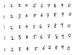
Most of the time we would like to automate our image pre-processing stage especially during the data extraction for database. In other words, the program should be able to extract the characters one by obe and map the target output for training purpose. The following code shows the example:

1. Read Image
This cell of codes read the image to MATLAB workspace

I = imread('sample.bmp');
imshow(I)

2. Convert to grayscale image
This cell of codes convert the RGB to gray

Igray = rgb2gray(I);
imshow(Igray)


3. Convert to binary image
This cell of codes convert the gray to binary image

Ibw = im2bw(Igray,graythresh(Igray));
imshow(Ibw)


4. Edge detection
This cell of codes detect the edge of the image

Iedge = edge(uint8(Ibw));
imshow(Iedge)

5. Morphology
This cell of codes perform the image dilation and image filling on the image

Image Dilation

se = strel('square',2);
Iedge2 = imdilate(Iedge, se);
imshow(Iedge2);


Image Filling

Ifill= imfill(Iedge2,'holes');
imshow(Ifill)


6. Blobs analysis
This cell of codes find all the objects on the image, and find the properties of each object.

[Ilabel num] = bwlabel(Ifill);
disp(num);
Iprops = regionprops(Ilabel);
Ibox = [Iprops.BoundingBox];
Ibox = reshape(Ibox,[4 50]);
imshow(I)

50


7. Plot the Object Location
This cell of codes plot the object locations

hold on;
for cnt = 1:50
rectangle('position',Ibox(:,cnt),'edgecolor','r');
end


By this, we are able to extract the character and pass to another stage for "classification" or "training" purpose. (To be continue...)

* MATLAB® is the registered trademarks for The MathWorks, Inc

The required files can be found at:
(link for the required files will be provided soon...)

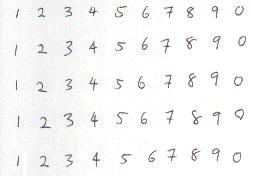
Character Recognition Example (I): Image Pre-processing

This example illustrates simple way of character recognition. It just serves as a kick start for beginers by introducing them simple coding in MATLAB for character recognition.

Some useful example for image pre-processing before the recognition stage is shown as follow:

1. Manual Cropping
This cell of codes allow the user to crop the image manually, which is important proccess especially the programmer would like to manipulate the data more in details.

img = imread('sample.bmp');
imshow(img)
imgGray = rgb2gray(img);
imgCrop = imcrop(imgGray);
imshow(imgCrop)


2. Resizing
This cell of codes magnify the image for 5 times. Resize function is important when the size of the character are not standard, especially in the handwritting recognition program.

imgLGE = imresize(imgCrop, 5, 'bicubic');
imshow(imgLGE)



3. Rotation
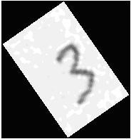
This cell of codes rotate the image for 35 degree. Some of the printed documents might not in the right degree as expected. This operation coulf make the character to our desired angle.

imgRTE = imrotate(imgLGE, 35);
imshow(imgRTE)



4. Binary Image
This cell of codes convert the image to binary image. Definitely, the speed and also the accuracy will increse if this operation is perform properly.

imgBW = im2bw(imgLGE, 0.90455);
imshow(imgBW)

Detecting Object in an Image

1. How to detect an object in an image?
Determining the features from the object that you want to detect is the key. The feature in this case is something that differentiates the object from others, such as color, shape, size, etc…

2. What are the techniques for object detection?
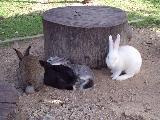
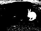
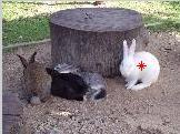
The image processing techniques such as morphology or color processing usually did this job. A simple example in MATLAB® of detecting ‘white rabbit’ is shown as follow, in this case, ‘color’ is the feature used to distinguish the white rabbit from other:

% Original Image
S = imread('pic3b.jpg');
imshow(S);

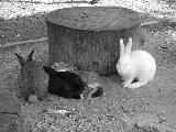
% Gray scale image
S2 = rgb2gray(S);
imshow(S2);

% Find the white color
S3 = S2>180;
imshow(S3);

% Morphology technique, image erosion to erase the unwanted components
se = strel('line',10,90);
S4 = imerode(S3,se);
se = strel('line',10,0);
S4 = imerode(S4,se);
imshow(S4)

% Labeled the component(s), and plot the centroid on the original image
S5 = bwlabel(S5);
[x,y]=find(S6==1);
imshow(S)
hold on;plot(mean(y),mean(x),'r*')

More information of image processing techniques can be found by searching "morphology", "morphological" from the search engine or the google search bar at the right hand site of this page.

* MATLAB® is the registered trademarks for The MathWorks, Inc

Drawing Shapes by Overwriting Pixel Value

1. How to highlight certain portion on an image?
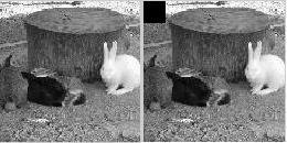
The basic concept of highlighting part of an image is “Overwriting Pixel Value” on the image. We start from the basic idea on how to mask portion of image with blank sub-image (black color sub-image). Fig 1 shows the image with the size of 128x128x3 in which 3 represent s RGB. (In grayscale image 3 layers are the same). The image at the right hand site shows a blank sub-image is placed at the upper left of the original image. The MATLAB® code to perform the operation are as follow:

S = imread('t3.jpg');
imshow(S);
Sblack = uint8(zeros(20,20,3));
S2 = S;
S2(1:20,1:20,:) = Sblack;
imshow(S2);

Fig 1

2. How to create a color mask rather than black color mask?
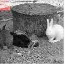
Since the 3 layers of image matrix represent RGB layers of the image, we can create the red color mask using following command, and the results are shown in fig 2.

Sred = Sblack;
Sred(:,:,1)=255;
S2 = S;
S2(1:20,1:20,:) = Sred;
imshow(S2);

Fig 2


3. How to create a transparent mask?
Simple enough, just play with the values R value, and perform the image addition rather than overwriting the value as follow:

Sred = Sblack;
Sred(:,:,1)=200;
S2 = S;
S2(1:20,1:20,:) = S2(1:20,1:20,:) + Sred;
imshow(S2);

Fig 3

4. Finally, how to create an outline for the image?

linelength = 10;
Sblack = uint8(zeros(128+linelength*2,128+linelength*2,3));
S2 = Sblack;
S2((1+linelength):(end-linelength),(1+linelength):(end-linelength),:)=S;
imshow(S2);

Fig 4

The “linelength” variable is the outline length in pixel.

* MATLAB® is the registered trademarks for The MathWorks, Inc

What is Image Compression?

This blog is not for the expert, but for those who like to ask, “what is..?” “how to..?” and “…so what?”. If you want the prove in the form of mathematic equations, this is not the right place you should come.

No mathematic equation will be shown, but prove of the methods and the basic concepts of an algorithm and how to apply it in research, work, or “just for fun”.

The very first topic that I would like to share is the concept of simple image compression. So the first question you might ask is:

1. What is image compression and how to perform image compression?
Image compression is the technique to compress the image to save storage space as well as before transmitting it through some transmission medium. The most common method of image compression is discrete cosine transform (DCT). By taking the DCT of an original image, the low frequencies contents will be transform into the upper left of the DCT matrix… why…? Don’t ask me why, again, this blob is just for those what want to know “how to…?” and “…so what?” but not for “why…?”. If you would like to learn more on the image compression, you can use any search engine, or you might want to use the Google search bar on the right panel of this page to search for the “image compression”. :)


2. So what after I know the DCT concept? How to apply this into image compression?
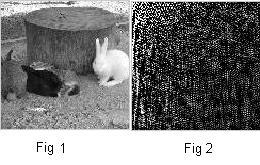
The low frequencies components, which also carry most of the information of the image, are our focus. The fig 1 shows the original image while fig 2 shows the DCT matrix for the image. Notice that the “white color” is concentrated at the upper left of the DCT matrix? That’s the “information (energy) for the image which also represents the low frequency components of the image. If we perform a inverse DCT for the fig 2, we will get back the fig 1.

3. How to compress the image?
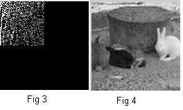
Fig 2 is the DCT matrix of the image. If we through away the high frequencies components, which contain not much information (dark color portion), we can achieve certain level of compression. For example, if I just take quarter of the DCT matrix, I save 75% of the storage!

4. So what is the tradeoff for this storage saving?
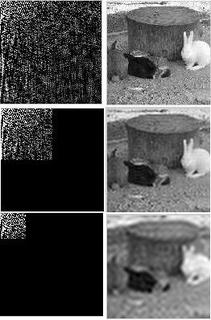
We will get some distortion of the image after the reconstruction of the image using the Inversed DCT as shown in fig 4. The level of the distortion is depends on the level of compression you choose. Some visual comparisons are shown in the following figures.

5. What software can I use to work on the above example?
You can use any search engine or the Google search bar on the right panel of this page and search for the “math software”, you would find numbers of useful softwares to perform this.