After preprocess the image, the training dataset is used to train "classification engine" for recognition purpose. In this example, a multi-layer feed-forward back-propagation Neural Network will be used.
1. Read the imageI = imread('sample.bmp');
2. Image PreprocessingThis cell of codes will extract all the components (objects) as descript in section II.
img = edu_imgpreprocess(I);
for cnt = 1:50
bw2 = edu_imgcrop(img{cnt});
charvec = edu_imgresize(bw2);
out(:,cnt) = charvec;
end
3. Creating Vectors data for the Neural Network (objects)These few line of codes creates training vector and testing vector for the neural network. This is to match the input accepted by the neural network function. The front 4 rows will be used to train the network, while the last row will be used to evaluate the performance of the network. (Please refer to part I and II for the dataset)
P = out(:,1:40);
T = [eye(10) eye(10) eye(10) eye(10)];
Ptest = out(:,41:50);
4. Creating and training of the Neural Network
Create and Train NN. The "edu_createnn" is a function file to create and train the network by accepting the training-target datasets
net = edu_createnn(P,T);
TRAINGDX, Epoch 0/5000, SSE 100.603/0.1, Gradient 46.9458/1e-006
TRAINGDX, Epoch 20/5000, SSE 38.3704/0.1, Gradient 1.1137/1e-006
TRAINGDX, Epoch 40/5000, SSE 39.4562/0.1, Gradient 0.485735/1e-006
TRAINGDX, Epoch 60/5000, SSE 39.5979/0.1, Gradient 0.387782/1e-006
TRAINGDX, Epoch 80/5000, SSE 39.6081/0.1, Gradient 0.387929/1e-006
TRAINGDX, Epoch 100/5000, SSE 39.5559/0.1, Gradient 0.445316/1e-006
TRAINGDX, Epoch 120/5000, SSE 39.2765/0.1, Gradient 0.758668/1e-006
TRAINGDX, Epoch 140/5000, SSE 35.941/0.1, Gradient 1.34484/1e-006
TRAINGDX, Epoch 160/5000, SSE 23.9786/0.1, Gradient 2.73872/1e-006
TRAINGDX, Epoch 180/5000, SSE 1.57322/0.1, Gradient 0.898383/1e-006
TRAINGDX, Epoch 196/5000, SSE 0.0909575/0.1, Gradient 0.0769913/1e-006
TRAINGDX, Performance goal met.
 5. Testing the Neural Network
Simulate the testing dataset
[a,b]=max(sim(net,Ptest));
disp(b);
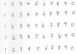
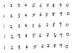
1 2 3 4 5 6 7 8 9 10
Do note that there might be some misclassifications on the simulated result with different training properties. The accuracy could be improved by better features extraction techniques as well as the selection of NN's properties.
* MATLAB® is the registered trademarks for The MathWorks, Inc
The relevant files can be found at:
(link to the files will be provided soon…)
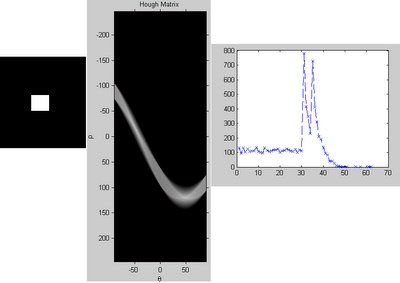
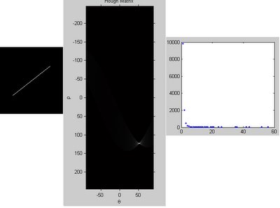
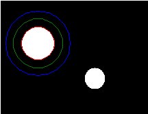
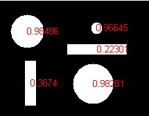
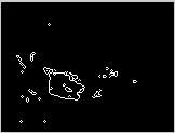
 For a round object, numbers of lines that cross 1 point, 2 points.....until n points in which n is the diameter of the round object (approximately) would be increase in exponently. This could be noticed in the right figure.
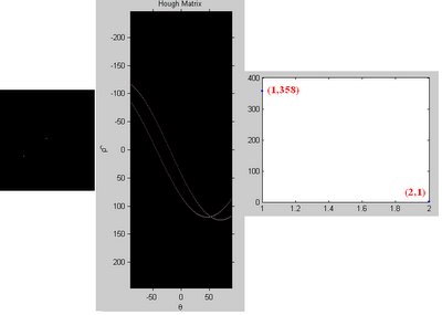


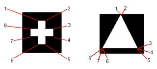 4. Ideally, a triangle will only have 3 extrema points. However, due to the imperfection of a binary object, a few of close-by points might exist instead of one.


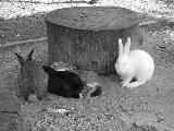
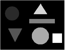
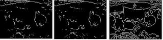 It seems like great but the usage of these output are useless until we really know what we want to do. For exmaple, we want to find the white rabbit, we need to perform some pre-processing before the edge detection so that we can fully utilize the function to suite to our needs.
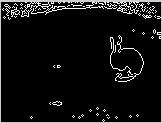
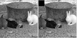
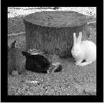
 The post processing can be used to remove unwanted noise.