Detecting Objects' Shape(II) : Square Object

Detecting square object could be done in similar way we used to detect the round object. What we need to know is just the the formula for the area and the perimeter of a square object which is A = w^2 and P = 4*w.


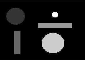
1. Original image and the negative image (value 0 represent background while 1 represent oject).
S = imread('pic10.jpg');
S = im2bw(S);
S2 = ~S;
imshow(S2);


2. Labeling the objects in the image. The advance programming language will support this function and label the objects.
S3 = bwlabel(S2);
imshow(S3,[]);

3. Some properties of the objects are extracted using the command. In this example, we just use the area and perimeter for our calculation.
S4 = regionprops(S3,'Area','Perimeter','centroid');

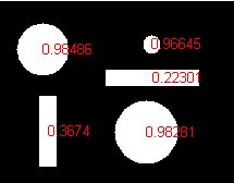
4. Now, evaluate the "squareness" of the objects. this is evaluated by only 1 criteria in this example:
a. Calculate the length or width of the object by using the formulas of area and perimeter, comparing the result and the square objects would have higher score than others. Do note that instead of for loop, the code below is a vectorized code.
score = (min(sqrt([S4.Area]),[S4.Perimeter]/4)./(max(sqrt([S4.Area]), ...[S4.Perimeter]/4))).^2;

5. Display the result visually
imshow(S2)
for cnt = 1:length(S4)
text(S4(cnt).Centroid(1),S4(cnt).Centroid(2),num2str(score(cnt)),'color','red');
end


Do note that this example assumes perfect images. For more accurate results, more properties can be compared by using more criteria. The example above is done using MATLAB®.


MATLAB® is registered trademarks of The MathWorks.

Detecting Objects' Shape(I) : Round Object

With the powerful technical computing language, the job of detection an object's shape no longer require lengthy codes. What important is the fundamental of mathematic that define the properties of the shape of objects. Let's look into the detection of round object in this section.

1. Original image and the negative image (value 0 represent background while 1 represents object).

S = imread('pic9.jpg');
S = im2bw(S);
S2 = ~S;
imshow(S2);




2. Labeling the objects in the image. The advance programming language will support this function and label the objects automatically.
S3 = bwlabel(S2);
imagesc(S3);



3. Getting the properties of the objects that require for calculation, which are: the longest and shortest diameter for the object, the area and the perimeter of the object, and the centroid of the object.
S4 = regionprops(S3,'MinorAxisLength','MajorAxisLength','Area','Perimeter','centroid');

4. Now, evaluate the "roundness" of the objects. this is evaluated by 3 criteria:
a. Comparing the longest and shortest diameter for the object,
b. Comparing the Area with the formula pi*r^2.
c. Comparing the Perimeter with the formula 2*pi*r
The "scores" are normalized so that 1 represent "best fit"

for cnt = 1:length(S4)
score1(cnt) = abs(1-(S4(cnt).MajorAxisLength-S4(cnt).MinorAxisLength)...
/max([S4(cnt).MajorAxisLength,S4(cnt).MinorAxisLength]));
score2(cnt) = abs(1 - abs(pi*((mean([S4(cnt).MajorAxisLength,...
S4(cnt).MinorAxisLength]))/2)^2-S4(cnt).Area)/S4(cnt).Area);
score3(cnt) = abs(1 - abs(pi*(max([S4(cnt).MajorAxisLength,...
S4(cnt).MinorAxisLength]))-S4(cnt).Perimeter)/S4(cnt).Perimeter);
end
score = mean([score1;score2;score3]);

5. Display the result visually

imshow(S2)
for cnt = 1:length(S4)
text(S4(cnt).Centroid(1),S4(cnt).Centroid(2),num2str(score(cnt)),'color','red');
end

Playing with “Edge Detection”

A lot of articles explain what is edge detection, how to apply it, and the usage of it. Different edge detection techniques such as sobel, prewitt, and canny are easily found from any image processing software.

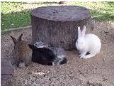
However, when we really want to perform edge detection for certain purpose, the problems arise. Look at the following example:

1. Original image
S = imread('pic8.jpg');
imshow(S);

2. Edge detection using different methods
S2 = rgb2gray(S);
figure,edge(S2,'sobel');
figure,edge(S2,'prewitt');
figure, edge(S2,'canny');

It seems like great but the usage of these output are useless until we really know what we want to do. For exmaple, we want to find the white rabbit, we need to perform some pre-processing before the edge detection so that we can fully utilize the function to suite to our needs.

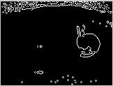
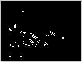
3. Edge detection for the white rabbit
Since we know the RGB value for white color is [255,255,255], we can pre-process the image to extract the white color region from the image.

Sw = S(:,:,1)>200 & S(:,:,2)>200 & S(:,:,3)>200;
edge(double(Sw));

Well, it seems like make more sense. Let's have a look on how to perform edge detection on the black rabbit:

4. Edge detection for the black rabbit

Sb = S(:,:,1)<40 & S(:,:,2)<40 & S(:,:,3)<40;

The post processing can be used to remove unwanted noise.

Panoramic Picture Creation

This example illustrates simple method of panoramic picture creation using sum of absolute differences. It assumes no zooming, rotational variation in 2 images.

1. Reading Images for processing
S1 = imread('p1.jpg');
S2 = imread('p2.jpg');

2. Showing Images
1st Image

imshow(S1);



2nd Image

imshow(S2);



3. Extract red layer of the image for processing using Sum of Absolute Differences (SAD)
S1r = S1(:,:,1);
S2r = S2(:,:,1);

4. Sum of Absolute Differences (SAD) of a selected block is from each image are computed.
sz = 50;
roi2 = S2r(1:sz,1:sz);
[x,y]=size(S2r);
for cnt = y:-1:x/2
roi1 = S1r(1:sz,cnt-sz+1:cnt);
data(y-cnt+1)=sum(sum(abs(double(roi2)-double(roi1))));
end

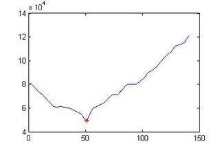
5. Finding minimum error among all comparison
plot(data)
[minval,ind] = min(data);
hold on;
plot(ind,minval,'r*');





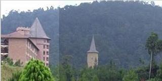
6. Combine the images at the minimum error region.
Sc = S1(1:end,1:y-sz-ind+1,:);
Sfinal = [Sc S2];

7. Final Result
figure;
imshow(Sfinal);

Character Recognition Example (III):Training a Simple NN for classification

After preprocess the image, the training dataset is used to train "classification engine" for recognition purpose. In this example, a multi-layer feed-forward back-propagation Neural Network will be used.

1. Read the image
I = imread('sample.bmp');

2. Image Preprocessing
This cell of codes will extract all the components (objects) as descript in section II.

img = edu_imgpreprocess(I);
for cnt = 1:50
bw2 = edu_imgcrop(img{cnt});
charvec = edu_imgresize(bw2);
out(:,cnt) = charvec;
end

3. Creating Vectors data for the Neural Network (objects)
These few line of codes creates training vector and testing vector for the neural network. This is to match the input accepted by the neural network function. The front 4 rows will be used to train the network, while the last row will be used to evaluate the performance of the network. (Please refer to part I and II for the dataset)

P = out(:,1:40);
T = [eye(10) eye(10) eye(10) eye(10)];
Ptest = out(:,41:50);

4. Creating and training of the Neural Network
Create and Train NN. The "edu_createnn" is a function file to create and train the network by accepting the training-target datasets

net = edu_createnn(P,T);

TRAINGDX, Epoch 0/5000, SSE 100.603/0.1, Gradient 46.9458/1e-006
TRAINGDX, Epoch 20/5000, SSE 38.3704/0.1, Gradient 1.1137/1e-006
TRAINGDX, Epoch 40/5000, SSE 39.4562/0.1, Gradient 0.485735/1e-006
TRAINGDX, Epoch 60/5000, SSE 39.5979/0.1, Gradient 0.387782/1e-006
TRAINGDX, Epoch 80/5000, SSE 39.6081/0.1, Gradient 0.387929/1e-006
TRAINGDX, Epoch 100/5000, SSE 39.5559/0.1, Gradient 0.445316/1e-006
TRAINGDX, Epoch 120/5000, SSE 39.2765/0.1, Gradient 0.758668/1e-006
TRAINGDX, Epoch 140/5000, SSE 35.941/0.1, Gradient 1.34484/1e-006
TRAINGDX, Epoch 160/5000, SSE 23.9786/0.1, Gradient 2.73872/1e-006
TRAINGDX, Epoch 180/5000, SSE 1.57322/0.1, Gradient 0.898383/1e-006
TRAINGDX, Epoch 196/5000, SSE 0.0909575/0.1, Gradient 0.0769913/1e-006
TRAINGDX, Performance goal met.




5. Testing the Neural Network
Simulate the testing dataset

[a,b]=max(sim(net,Ptest));
disp(b);

1 2 3 4 5 6 7 8 9 10



Do note that there might be some misclassifications on the simulated result with different training properties. The accuracy could be improved by better features extraction techniques as well as the selection of NN's properties.

* MATLAB® is the registered trademarks for The MathWorks, Inc

The relevant files can be found at:
(link to the files will be provided soon…)