Hough Transform For Hyperbola Detection - with known eccentricity

More Hough Transform examples!

In last few examples, the Hough Transform are used to detect different shape, such as line and circle. For the circle detection, examples of circles with known radius detection and circles with unknown radius detection have been illustrated.

Besides, different techniques of implemeting the code are shown, as in "for" loops and vectorized code.

In this example, example of how the Hough Transform could be used for hyperbola detection would be demonstrated.

Firstly, let's see the equation of the hyperbola:

(x-xo)^2/a^2 - (y-yo)^2/b^2 = 1

Let's start with a simple example to find the asymptotes and the crossing point of a hyperbola with known eccentricity, e^2 = a^2 + b^2, and to simplified the problem, let's make the a = b = 29.

1. Reading image and the convert to binary image. After that, the location of the value '1' is found using 'find' function. (the image is in white background and black object, so the '~' is used to get the negative image.

clear all;clc;
I = imread('pic27.bmp');
I =im2bw(I);
imshow(I);
I = ~I;
[y,x]=find(I);
[sy,sx]=size(I);
imshow(I);

2. Find all the require information for the transformatin. the 'totalpix' is the numbers of '1' in the image

totalpix = length(x);

3. Preallocate memory for the Hough Matrix. In this case, the a and b are known as 29 (in pixels).

HM = zeros(sy,sx);
a = 29;
b = 29;

4. Performing Hough Transform to transform the x-y domain to xo-yo domain.

yo = 1:sy;

for cnt = 1:totalpix


% a. Four lines of equation here to detect the hyperbola shapes in 4
% different direction
xo(:,1) = round(x(cnt) + sqrt(a.^2.*(((y(cnt)-yo).^2/(b.^2))+1)));
xo(:,2) = round(x(cnt) - sqrt(a.^2.*(((y(cnt)-yo).^2/(b.^2))+1)));
xo(:,3) = round(x(cnt) + sqrt(a.^2.*(((y(cnt)-yo).^2/(b.^2))-1)));
xo(:,4) = round(x(cnt) - sqrt(a.^2.*(((y(cnt)-yo).^2/(b.^2))-1)));


% b. Since there are 4 equations, Hough Matrix must consists of the
% combination for 4 equation.
for cnt3 = 1:4
for cnt2 = 1:sy

HM(cnt2,xo(cnt2,cnt3)) = HM(cnt2,xo(cnt2,cnt3)) + 1;

end
end
end

end

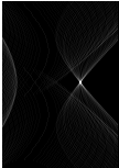
5. Showing the Hough Matrix

imshow(HM,[]);

6. Finding the asymptotes and the crossing point of a hyperbola

[maxval, maxind] = max(max(HM));
[Yo,Xo] = find(HM==maxval);
imshow(I); hold on;
plot(mean(Xo),mean(Yo),'xr')
c1 = mean(Yo) - mean(Xo);hold on;
plot(1:100, [1:100] + c1);
c2 = mean(Yo) + mean(Xo); hold on;
plot(1:100, -[1:100] + c2);

Y = 1:sy;
X = -sqrt(((Y-mean(Yo)).^2/a.^2 + 1).*b.^2) + mean(Xo);
hold on;
plot(X,real(Y),'r');

Hough Transform For Circle Detection - with unknown radius (II)

The detection of circle with unknown radius has been shown in previous post - Hough Transform For Circle Detection - with unknown radius (I) , by using a lot of "for" loops.

This example shows the same function with "vectorized" code, which run 25% faster than the previous code, in a Pentium M 1.5 GHz computer with 512 M RAM.

Let's see how to perform this:

1. Reading image and the convert to binary image. After that, the location of the value '1' is found using 'find' function. (Assume the image is already preprocess, if not, the 'edge' function might help)

clear all;clc;
I = imread('pic26.bmp');
I =im2bw(I);
[y,x]=find(I);
[sy,sx]=size(I);
imshow(I);



2. Find all the require information for the transformation. The 'totalpix' is the numbers of '1' in the image.

totalpix = length(x);

3. Pre-allocate memory for the Hough Matrix and other variables. The ‘R’ is known in the range from 1 to 50, so we reserve 50 "layers" for the HM matrix.

HM = zeros(sy*sx*50,1);
R = 1:50;
R2(1,1,:) = R.^2;
R2 = repmat(R2,[sy,totalpix,1]);
y = repmat(y',[sy,1,50]);
x = repmat(x',[sy,1,50]);
b = 1:sy;
b = repmat(b',[1,totalpix,50]);
a = zeros(sy,totalpix);

4. Performing Hough Transform. Do notice that no "for" loops are used here.

a. Find the a parameter

a = (round(x - sqrt(R2 - (y - b).^2)));

b. Find the location of ‘a’ and ‘b’, as well as the valid value both.

[xx,yy,zz]=find((imag(a)==0 & a>0));
b = b(imag(a)==0 & a>0);
a = a(imag(a)==0 & a>0);

c. Find the indices and remap it to different layers

ind = sub2ind([sy,sx],b,a);
ind = ind + (ceil(yy/totalpix)-1)*sx*sy;

d. Construct the Hough Matrix of 50 layers

val = ones(length(ind),1);
data=accumarray(ind,val);
HM(1:length(data)) = data;
HM2 = reshape(HM,[sy,sx,50]);

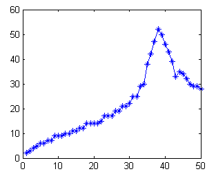
5. Find for the maximum value for each layer, or in other words, the layer with maximum value will indicate the corresponding ‘R’ for the circle.

for cnt = 1:50
H(cnt) = max(max(HM2(:,:,cnt)));
end
plot(H,'*-');



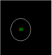
6. Extract the information from the layer with maximum value, and overlap with the original image.

[maxval, maxind] = max(H);
[B,A] = find(HM2(:,:,maxind)==maxval);
imshow(I); hold on;
plot(mean(A),mean(B),'xr')
text(mean(A),mean(B),num2str(maxind),'color','green')


7. This example use the vectorized code, and the speed of the program is 25 % faster than the previous example using "for" loops.

Fill The Area Between 2 Lines

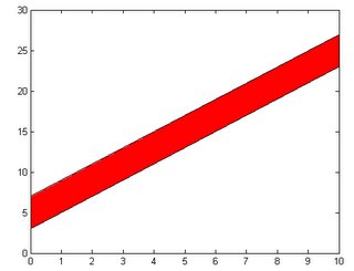
This example shows how to fill the area between 2 lines with color.

1. Assuming we have two lines on a plot

x1 = 0:10;
y1 = 2*x+3;
y2 = 2*x+7;
plot(x,y1);
hold on;
plot(x,y2);



2. One of the simple way to fill the are between 2 lines is:

a. Find 4 points for the 2 lines - start point and end point, assuming 2 lines are within certain boundary, so the x vector will be (do note that the points must be defined in order, either clock-wise or anti clock-wise):

x = [0 10 10 0];

b. Replacing x in to y1 and y2 to get y vector:

y = [3 23 27 7];

3. Use the "fill" or "patch" function to fill the area between 2 lines.

patch(x,y,'r')