Converting Pixels to Line

Converting pixels to line could be a complicated job. A simple example is shown to serve as the basis of a complicated problem.

1. Reading image

clear all;clc;
I = imread('pic24.jpg');
I = im2bw(I);
imshow(I);

2. Finding all the pixels with the value of '1'

[y,x] = find(I==1);
imshow(I);
hold on;
plot(x,y);



3. Use the "polyfit" function to fit polynomial to data, in our case, since it is a straight line, we use 1st order polynomial or a linear equation Y = M*X + C

p = polyfit(x,y,1);
disp(p);

-0.7873 158.3164


4. Find the image size and create the X and Y based on the coefficients of "p".

sz = size(I);
X = 1:sz(2);
Y = p(1) * X + p(2);

5. Display the result

imshow(I);
hold on;
plot(X,Y);

Detecting Objects' Motion in 2 Subsequence Images

I've been posting examples of Hough Transform since last month, and now is the time to switch to other examples.

1. Reading image and comparing 2 images side by side

clear all;clc;
Ia = imread('pic23a.jpg');
Ib = imread('pic23b.jpg');
subplot(121);imshow(Ia);
subplot(122);imshow(Ib);













2. Finding the location of green object in 2 images

a. Set the threshold value for green color




p/s: I can't make the "&" appear in text, so the text aboved is in image format.

b. Find the location of the green object

[y1,x1] = find(Ia_green==1);
[y2,x2] = find(Ib_green==1);

c. Find the centroid of the green object

x1 = round(mean(x1));
y1 = round(mean(y1));
x2 = round(mean(x2));
y2 = round(mean(y2));


3. Putting 2 images together and show the movement of the objects

figure;
imshow(Ia); hold on;
imshow(Ib);
alpha(.5);
plot(x1,y1,'r*');
plot(x2,y2,'ro');
plot([x1,x2],[y1,y2]);





The '*' indicates the start point of the object while the 'o' is the stop point of the object. Other objects' movement could be found by modifying the step number 2.

Hough Transform For Circle Detection - with unknown radius (I)

In previous 2 examples, the generalized Hough Transform has been applied to find for the circle with known radius. We were using the circle equation --> (x-a)^2 + (y-b)^2 = R^2 to map the pixel to a-b domain.

For detection circle with unknown radius, another parameter need to be make as variable, which is, the radius R.

Let's see how to perform this:

1. Reading image and the convert to binary image. After that, the location of the value '1' is found using 'find' function. (assume the image is already preprocess, if not, the 'edge' function might help)

clear all;clc;
I = imread('pic22.bmp');
I =im2bw(I);
[y,x]=find(I);
[sy,sx]=size(I);
imshow(I);


2. Find all the require information for the transformatin. the 'totalpix' is the numbers of '1' in the image.

totalpix = length(x);

3. Preallocate memory for the Hough Matrix. The R is known in the range from 1 to 50, so we reserve 50 "layers" for the HM matrix.

HM = zeros(sy,sx,50);
R = 1:50;
R2 = R.^2;
sz = sy*sx;

4. Performing Hough Transform. Notice the accumulator is located in the inner for loop.

for cnt = 1:totalpix
for cntR = 1:50
b = 1:sy;
a = (round(x(cnt) - sqrt(R2(cntR) - (y(cnt) - [1:sy]).^2)));
b = b(imag(a)==0 & a>0);
a = a(imag(a)==0 & a>0);
ind = sub2ind([sy,sx],b,a);
HM(sz*(cntR-1)+ind) = HM(sz*(cntR-1)+ind) + 1;
end
end

5. Find for the maximum value for each layer, or in other words, the layer with maximum value will indicate the correspond R for the circle.

for cnt = 1:50
H(cnt) = max(max(HM(:,:,cnt)));
end
plot(H,'*-');



6. Extract the information from the layer with maximum value, and overlap with the original image.

[maxval, maxind] = max(H);
[B,A] = find(HM(:,:,maxind)==maxval);
imshow(I); hold on;
plot(mean(A),mean(B),'xr')
text(mean(A),mean(B),num2str(maxind),'color','green')


7. This example use the "for loop" extensively, and the speed of the program is rather slow. Vectorized the code might speed up the execution time, we wee see it in the next example. :)

Hough Transform For Circle Detection - with known radius (II)

This example doing the same as the previous example, with the difference that this example does not use any "for loops" in the code. The vectorized code make the algorithm runs faster but with the trade-off of high memory consumtion. Try to compare this with the previous example:

1. Reading image and the convert to binary image. After that, the location of the value '1' is found using 'find' function. (assume the image is already preprocess, if not, the 'edge' function might help)

clear all;clc;
I = imread('pic21.bmp');
I =im2bw(I);
[y,x]=find(I);
[sy,sx]=size(I);
imshow(I);

2. Find all the require information for the transformatin. the 'totalpix' is the numbers of '1' in the image.

totalpix = length(x);

3. Preallocate memory for the Hough Matrix. Try to play around with the R, or the radius to see the different results.

HM = zeros(sy*sx,1);
R = 36;
R2 = R^2;

4. Performing Hough Transform. Notice that no "for-loop" in this portion of code.

a. Preparing all the matrices for the computation without "for-loop"

b = 1:sy;
a = zeros(sy,totalpix);

y = repmat(y',[sy,1]);
x = repmat(x',[sy,1]);

b = repmat(b',[1,totalpix]);

b. The equation for the circle

a = (round(x - sqrt(R2 - (y - b).^2)));

c. Removing all the invalid value in matrices a and b

b = b(imag(a)==0 & a>0);
a = a(imag(a)==0 & a>0);
ind = sub2ind([sy,sx],b,a);

d. Reconstruct the Hough Matrix

val = ones(length(ind),1);
data=accumarray(ind,val);
HM(1:length(data)) = data;
HM2 = reshape(HM,[sy,sx]);

5. Showing the Hough Matrix
cla
imshow(HM2,[]);

6. Finding the location of the circle with radius of R

[maxval, maxind] = max(max(HM2));
[B,A] = find(HM2==maxval);
imshow(I); hold on;
plot(mean(A),mean(B),'xr')

Hough Transform For Circle Detection - with known radius (I)

Some examples using Hough Transform are shown in previous few examples. Firstly, we have look into how to use standard Hough Transform function from new version of image processing toolbox to classified different objects.(Refer to Object Detection using Hough Transform (I) and (II) ) Secondly, we have look into how to implement our own code for Hough Transform (Refer to Simple Code for Hough Transform).

The second approach would be more flexible especially when we want to modified the Hought Transform to detect other shape other than line. In this example, a modified version of Hough Transform is used to detect the circle instead of line.

In this case, instead of transforming the pixel to rho and theta domain, we use the circle equation --> (x-a)^2 + (y-b)^2 = R^2 to map the pixel to a-b domain. Let's see how to perform this:

1. Reading image and the convert to binary image. After that, the location of the value '1' is found using 'find' function. (assume the image is already preprocess, if not, the 'edge' function might help)

clear all;clc;
I = imread('pic20.bmp');
I =im2bw(I);
[y,x]=find(I);
[sy,sx]=size(I);
imshow(I);

2. Find all the require information for the transformatin. the 'totalpix' is the numbers of '1' in the image.

totalpix = length(x);

3. Preallocate memory for the Hough Matrix. Try to play around with the R, or the radius to see the different results.

HM = zeros(sy,sx);
R = 34;
R2 = R^2;

4. Performing Hough Transform. Notice the accumulator is located in the inner for loop. This portion of codes will map the original image to the a-b domain.

b = 1:sy;

for cnt = 1:totalpix
a = (round(x(cnt) - sqrt(R2 - (y(cnt) - [1:sy]).^2)));
for cnt2 =1:sy
if isreal(a(cnt2)) & a(cnt2)>0
HM(cnt2,a(cnt2)) = HM(cnt2,a(cnt2)) + 1;
end
end
end

5. Showing the Hough Matrix

imshow(HM,[]);






6. Finding the location of the circle with radius of R

[maxval, maxind] = max(max(HM));
[B,A] = find(HM==maxval);
imshow(I); hold on;
plot(mean(A),mean(B),'xr')

Simple Code for Hough Transform

Previous few examples using the Hough Transform function to perform the operation. However, Hough Transform function only available in new version of the tools. For those who are still using older version, this example shows a simple way of performing Hough Transform with a few lines of codes.

1. Reading image and the convert to binary image. After that, the location of the value '1' is found using 'find' function. (assume the image is already preprocess, if not, the 'edge' function might help)

I = imread('pic20.jpg');
I =im2bw(I);
[y,x]=find(I);
[sy,sx]=size(I);
imshow(I);



2. Find all the require information for the transformatin. the 'totalpix' is the numbers of '1' in the image, while the 'maxrho' is used to find the size of the Hough Matrix

totalpix = length(x);
maxrho = round(sqrt(sx^2 + sy^2));

3. Preallocate memory for the Hough Matrix. The resolution for both rho and theta are set to one.

HM = zeros(2*maxrho,180);

4. Performing Hough Transform. Notice the accumulator is located in the inner for loop.

for cnt = 1:totalpix
cnt2 = 1;
for theta = -pi/2:pi/180:pi/2-pi/180
rho = round(x(cnt).*cos(theta) + y(cnt).*sin(theta));
HM(rho+maxrho,cnt2) = HM(rho+maxrho,cnt2) + 1;
cnt2 = cnt2 + 1;
end
end

theta = rad2deg(-pi/2:pi/180:pi/2-pi/180);
rho = -maxrho:maxrho-1;
imshow(uint8(HM),[],'xdata',theta,'ydata',rho);
xlabel('\theta'),ylabel('\rho')
axis on, axis normal;
title('Hough Matrix');


5. Done! However, the code is quite slow, anyway, it works!

Signature of Binary Objects

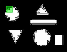
This example illustrates a simple way of converting the boundary of binary object into a 1-dimentional representation, or signature. One of the purpose of this conversion is to reduce the complexity of the representation for classification purpose. Let's have a look on how to convert the object to signature and compare the signature for different object shapes.

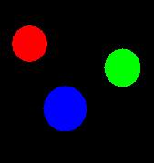
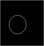
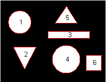
1. Original image (value 0 represent background while 1 represents object).

S = imread('pic19.jpg');
S = im2bw(S);
imshow(S);

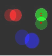
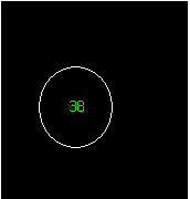
2. Get the boundary and plot them on top of the original image.

[B,L,N,A] = bwboundaries(S);
imshow(S);
for cnt = 1:N
hold on;
boundary = B{cnt};
plot(boundary(:,2), boundary(:,1),'r');
hold on;
text(mean(boundary(:,2)), mean(boundary(:,1)),num2str(cnt));
end


figure;
subplotrow = ceil(sqrt(N));

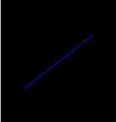
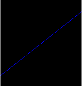
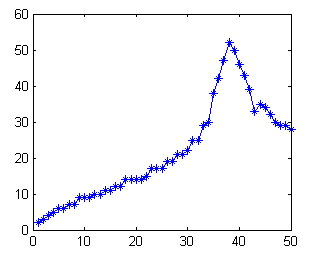
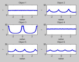
3. Plot the signature of each object.

for cnt = 1:N
boundary = B{cnt};
[th, r]=cart2pol(boundary(:,2)-mean(boundary(:,2)), ...
boundary(:,1)-mean(boundary(:,1)));
subplot(subplotrow,N/subplotrow,cnt);
plot(th,r,'.');
axis([-pi pi 0 50]);
xlabel('radian');ylabel('r');
title(['Object ', num2str(cnt)]);
end


More details explanation could be found from the image processing reference book which could be found at the site bar of this page